Desicion Trees are a non-parametric supervised learning method used for classifcation and regression. The goal is to create a model that predicts the value of a target variable by learning simple decision rules inferred from the data.
1. What is a Decision Tree? How does it work?
Decision tree is a type of supervised learning algorithm (having a pre-defined target varialbe) that is mostly used in classification problems. It works for both categorical and continous input and output variables. In this technique, we split the population or sample into two or more homogeneous sets based on most significant splitter in input variables.
Important terminology related to decision tree
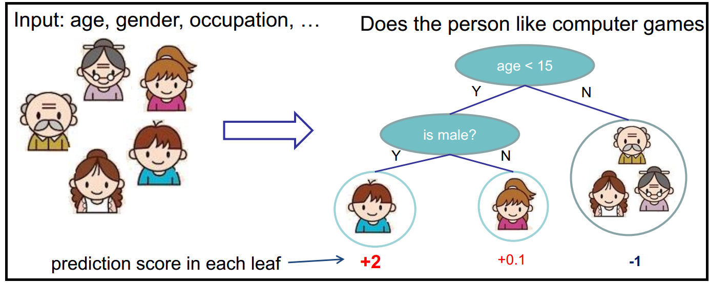
- Leaf/Terminal Node: nodes do not split is called leaf node.
- Decision Node: decision node is a question on features, it branches out according to answers.
- Pruning: when we remove the sub-nodes of a decison node, this process is called pruning. You can say opposite process of splitting.
Advantages
- Simple to understand and to interpret. Trees can be visulized.
- Requires little data preparation. It requires less data cleaning compared to some other modeling technique.
- Able to handle both numerical and categorical data.
- No parametric method. Decision tree is considered to be a non-parametric method. This means that decision tree have no asumption about space distribution and the classfier structure.
Disadvantages
- Overfitting. Decision tree can create over complex tree that do not generalize the data well.
2. How to build the tree?
The decision of making strategic splits heavily affects a tree's accuracy. There are many measures that can by used to determine the best way to split the samples. The creation of sub-nodes increases the homogeneity of resultant sub-nodes. In other words, we can say that purity of the node increases with respect to the target variables. Decision tree splits the nodes on all available variables and then selects the split which results in most homogeneous sub-nodes.
Let \(p(i/t)\) denote the fraction of samples belonging to class \(i\) at a given node \(t\).
Gini index
- a. calcuate Gini for sub-nodes, using the formula. \(Gini(t)=1-\sum[p(i/t)]^2\)
- b. calculate Gini for split using weighted Gini score of each node of that split.
Information gain
- a. calcuate entropy of parent node, using the formula. \(Entropy(t)=-\sum p(i/t)log_2p(i/t)\)
- b. calculate entropy of each individual node of split and calculate weighted average of all sub-nodes available in split.
Reduction in variance
Reduction in variance is an algorithm used for continuous target variables (regression problems).
- a. calcuate variance for each node. \(Variance=\frac{\sum (X-\bar{X})^2}{n}\)
- b. calculate variance for each split as weighted average of each node variance.
Missing values
Missing values are one of the curses of statistical models and analysis. Most procedure deal with them by refusing to deal with them - incomplete observations are tossed out.
Classification tree have a nice way to handling missing values by surrogate splits. To think about what to do if the splitted variable is not there. Classification trees tackle the issue by finding a replacement split. to find another split based on another variable, classification trees look at all the splits using all the other variables and search for the one yielding a division of training data points most similar to the optimal split.
3. How to avoid overfitting in decision tree?
Overfitting is one of the key challenges faced while modeling decision tree. If there is no limit set of a decision tree, it will give 100% accuracy on training set because in the worset case it will end up making 1 leaf node for each observation. Thus, preventing overfitting is pivotal while modeling a decision tree and it can be done in 2 ways.
- a. Setting constraints on tree size.
- b. Tree pruning.
Setting constraints on tree size
- a. Minimum samples for a node split Defines the minimum number of samples which are required in a node to be considered for splitting. It should be tuned using cross validation.
- b. Minimum samples for a terminal node Defines the minimum samples required in a terminal node or leaf.
- c. Maximum depth of tree The maximum depth of a tree. It should be tuned using cross validation.
- d. Maximum number of terminal nodes The maximum number of terminal nodes or leaves in a tree. Can be defined in place of max_depth. Since binary tree are created, a depth of 'n' would produce a maaximum of 2^n leaves.
- e. Maximum features to consider for split The number of features to consider while searching for a best split. These will be randomly selected. As a thumb-rule, square root of the total number of features works great but we should check upto 30%-40% of the total number of features.
Pruning the tree by cross-validation
- a. Use recursive binary splitting to grow a large tree on the training data. Stopping only when each terminal node has fewer than some minimum number of observations (This is to get a fully graown tree).
- b. Apply cost complexity pruning to the large tree in order to obatin a sequare of best subtree as a function of \(\alpha\).
\(R_\alpha(T)=R(T)+\alpha|T|\), we will define the tree complexity as \(|T|\), the number of terminal nodes in T. Let \(\alpha>0\) be a real number called complexity parameter. - c. Use K-fold cross validation to choose \(\alpha\), for each \(k=1...K\)
I. Repeat step a and b on the \(\frac{K-1}{K}\)th fraction of training data set excluding the \(K\)th fold.
II. Evaluate the mean squared prediction error on the data in the left-out \(K\)th fold as a function of \(\alpha\).
Average the results, and pick \(\alpha\) to minimize the average error. - d. Return the subtree from step b that corresponds to the choose value of \(\alpha\).
3. What is random forest? and How it works?
The literally meaning of word 'ensemble' is group. Ensemble methods involve group of predictive models to achieve a better accuracy and model stability. Ensemble methods are known to impart supreme boost to tree based models.
Bagging is technique used to reduce the variance of our predictions by combining the result of multiple classifiers modeled on different sub-samples of the same data set.
Random forest is considered to be a panacea of all data sceience problems. Random forest is a versatile learning method capable of performing both regression and classification tasks. It is a type of ensemble learning method, where a group of weak models combine to form a powerful model.

- a. Draw \(n_{tree}\) bootstrap samples from the original data.
- b. For each of the bootstrap samples, grow an unpruned classification or regression tree, with the following modification: at each node, rather than choosing the best split among all predictors, randomly sample \(m_{try}\) of the predictors and choose the best split from among those variables. (Bagging can be thought of as the special case of random forest obtained when \(m_{try}=p\), the number of predictors.)
- c. Predict new data by aggregating the predictions of the \(n_{tree}\) trees (i.e. majority votes for classification, average for regression).
- d. Return the subtree from step b that corresponds to the choose value of \(\alpha\).
An estimate of the error rate can be obtained based on the training data, by the following:
- a. At each bootstrap iteration, predict the data not in the bootstrap sample (what Breiman calls "out-of-bag" or OOB) using the tree grown with the bootstrap sample.
- b. Aggregate the OOB predictions. (On average, each data point would be OOB around 36% fo the times, so aggregate these predictions). Calculate the error rate, and call it the OOB estimate of error rate.
3. What is boosted tree?
Idea: given a weak learner, run it multiple times on (reweighted) training data, then let the learned classifiers vote.
On each iteration:
Final classifier: a linear combination of the votes of the different classifiers weighted by their strength.
Consider a weighted dataset:
- \(i\)th training example counts as \(D(i)\) examples.
- If I were to "resample" data, I would get more samples of "heavier" data samples.
- Given \((x_1,y_1),...,(x_m,y_m)\), where \(x_i \in X, y_i \in Y =\{-1,+1\}\). Initialize \(D_i(i)=1/m\).
- For \(t = 1,...,T:\)
- Train weak learner using distribution \(D_t\).
- Get weak classifier \(h_t: X \to R\).
- Choose \(\alpha_t \in R\).
- Update: \(D_{t+1}(i)=\frac{D_t(i)exp(-\alpha_t y_i h_t(x_i))}{Z_t}\) where \(Z_t \in R\) is a normalization factor \(Z_t =\sum^{m}_{i=1}D_t(i)exp(-\alpha_t y_i h_t(x_i))\)
- Output the final classifier: \(H(x)=sign(\sum^T_{t=1}\alpha_t h_t(x))\)
- \(\alpha_t = \frac{1}{2}ln(\frac{1-\epsilon_t}{\epsilon_t})\) \(\epsilon_t = \sum^m_{i=1}D_t(i)\delta(h_t(x_i)\neq y_i)\)