The Annotated Faster RCNN with PyTorch
from IPython.display import Image
Image(filename='image/fasterrcnn.jpg')
Faster RCNN is initially published in NIPS 2015, which serves as an intuitive speedup solution for the popular RCNN object detection algorithms.
In this blog, I present an "annotated" version of the paper in the form of line-by-line implementation.
Preliminary: import libraries
import numpy as np
import torch
import torch.nn as nn
import torch.nn.functional as F
import torchvision
from torchvision.ops import nms
import math, copy, time
from torch.autograd import Variable
import matplotlib.pyplot as plt
import seaborn
import cv2
import itertools
from utils import *
seaborn.set_context(context="talk")
%matplotlib inline
%load_ext autoreload
%autoreload 2
Table of Content
Background 
Recent advances in object detection are driven by the success of region proposal methods and region-based convolutional neural network (R-CNNs). Although region-based CNNs were computationally expensive as original developed, their cost has been drastically reduced thanks to the convolutions shared by proposals.
In RCNN and Fast-RCNN algorithm, selective search is used for region proposal, which greedily merges superpixels based on engineered low-level features. Compared with efficient detection networks in Fast RCNN, the selective search method is an order of magnitude slower.
The Faster RCNN shows an algorithmic change - computing proposals with a deep convolutional neural network - leads to an elegant and effective solution where proposal computation is nearly cost-free given the detection network's computation. To this end, the paper introduces Region Proposal Network (RPN) that share convolution layers with object detection network. By sharing convolutions at inference-time, the marginal cost for computing proposals is small.
Model Architecture 
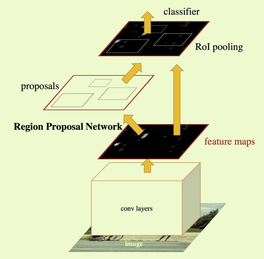
Faster RCNN is composed of two modules. The first module is a deep fully convolutional network that proposes regions, and the second module is the Fast R-CNN detector that uses the proposed regions. Then entire system is a single, unified network for object detection as shown in Fig 1.

Figure.1 Faster RCNN Architecture
Region Proposal Networks
The Region Proposal Networks (RPN) takes an image (of any size) as input and output a set of rectangular object proposals, each with an objectness score. Because the ultimate goal is to share computation with Fast R-CNN object detection network, the paper assumes that both nets share a common set of convoluation layers. In the paper, the author investigates ZF, which has 5 sharable convoluational layers and VGG-16 which has 13 sharelable layers. Since the inception of Faster RCNN, there are numerous noval network invented, which demonstrate better performance on ImageNet competition, such MobileNet, ResNet.
In this blog, we will use VGG-16 as base network for feature extractor.
original_model = torchvision.models.vgg16(pretrained=True)
device = torch.device("cuda" if torch.cuda.is_available() else "cpu")
class VGG16():
    """
    Use VGG-16 base network as feature extractor and classifer as RPN head
    Params:
        feature_level: feature level of vgg base network used for feature extractor
        freeze_level: feature level to be freezed, no need to further training
        use_drop: for the classifier, whether use the dropout layer in RPN head
    """
    def __init__(self, feature_level=30, freeze_level=10, use_drop=False):
        self.feature_level = feature_level
        self.freeze_level = freeze_level
        self.use_drop = use_drop
    def create_architecture(self):
        features = list(original_model.features)[:self.feature_level]
        classifier = list(original_model.classifier)[:6]

        if not self.use_drop:
            del classifier[5]
            del classifier[2]

        classifer = nn.Sequential(*classifier)

        for layer in features[:self.freeze_level]:
            for p in layer.parameters():
                p.requires_grad = False
        return nn.Sequential(*features), classifier
vgg = VGG16()
fmap, classifier = vgg.create_architecture()
# print the network architecture for base network
print(fmap)
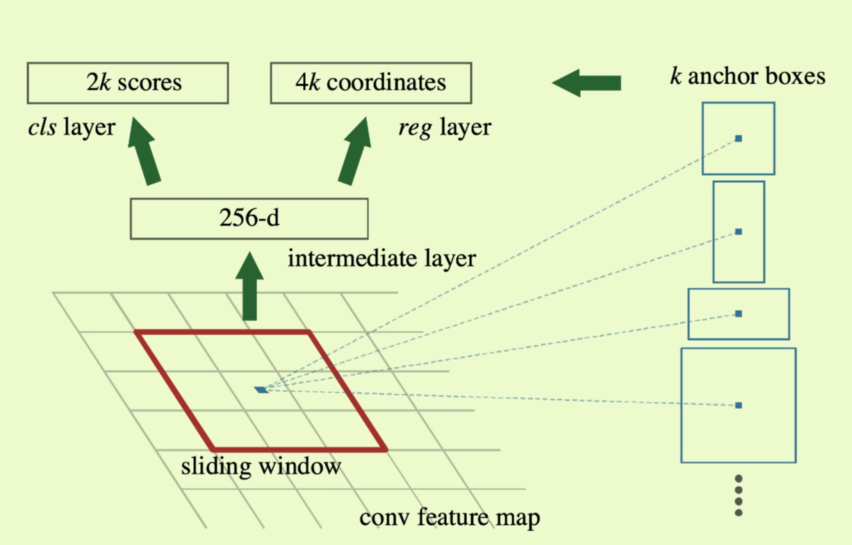
To generate region proposals, we slide a small network over the convolutional feature map output by the last shared convolutional layer. This small network takes as input an $n \times n$ spatial window of the input convolutional feature map. Each sliding window is mapped to a lower-dimensional feature (512-d for VGG with ReLU following). This feature is fed into two sibling fully connected layers - a box-regression layer ($reg$) and a box-classification layer ($cls$). This paper uses $n=3$.
Anchors
At each sliding-window location, we simultaneously predict multiple region proposals, where the number of maximum possible proposal for each location is denoted as $k$. So the $reg$ layer has $4k$ outputs encoding of $k$ boxes, and the $cls$ layer outputs $2k$ scores that estimate probability of object or not object for each proposal. The $k$ proposals are parameterized relative to $k$ reference boxes, which we call $anchors$. An anchor is centered at the sliding window in question, and is associated with a scale and aspect ratio. By default, we use 3 scales and 3 aspect ratio, yielding $k=9$ anchors at each sliding position.

Figure 2: Region Proposal Network (RPN)
If the feature map dimension is $conv_{width}\times conv_{height} \times conv_{height}$, the algorithm will create a set of anchor boxes for each of feature cell in $conv_{width} \times conv_{height}$. Even the anchor boxes are defined according to the dimension of feature map, all property of anchor boxes (location, scale etc) reference to the original image.
From the structure of base network above, the feature extractor (base network) only has convolutional, pooling and ReLu activition layers. Each pooling layer from VGG-16 network will reduce the dimension by half. Therefore, the dimensions of feature map are proportional to those of original image. For example, if the dimension of original image is $w\times h$, the feature map will be $\frac{w}{r}\times\frac{h}{r}$, where $r$ is the subsampling ratio. If we create a set of anchor boxes for each feature cell for the entire feature map, we will get multiple sets of anchor boxes separated by $r$ pixels.
def create_anchor_boxes(feature_h, feature_w, base_size=16, ratios=[0.5, 1, 2], anchor_scales=[8,16,32]):
    """
    Create anchor boxes that are scaled and modified to the given asepect ratio

    Params:
        base_size: the width and height of the reference box
        ratio: ratio of widht and height of the anchors
        anchor_scales: this is the scale of anchors compared with reference box size
        feature_h: height of feature map
        feature_w: width of feature map
    Returns:
        anchor_base: each element if a set of coordinates of a bounding box [y_min, m_min, y_max, x_max] for the feature cell
    """
    centerx = base_size/2
    centery = base_size/2

    anchor_base = []

    for s in anchor_scales:
        bbox_size = base_size*s
        for ar in ratios:
            h = bbox_size*np.sqrt(ar)
            w = bbox_size/np.sqrt(ar)
            anchor_base+= [[centery-h//2, centerx-w//2,centery+h//2, centerx+w//2]]

    anchor_base = np.array(anchor_base)

    # as explained, the anchor boxes are created according to feature map, but they reference to
    # original image
    cells_y = torch.arange(0, feature_h*base_size, base_size)
    cells_x = torch.arange(0, feature_w*base_size, base_size)

    cells_x, cells_y = np.meshgrid(cells_x, cells_y)
    cells_xy = np.stack((cells_y.ravel(), cells_x.ravel(), cells_y.ravel(), cells_x.ravel()), axis=1)

    num_anchorbox_reference = anchor_base.shape[0]
    num_cells = cells_xy.shape[0]

    anchor_boxes = anchor_base.reshape((1, num_anchorbox_reference, 4)) + cells_xy.reshape((1, num_cells, 4)).transpose((1,0,2))
    anchor_boxes = anchor_boxes.reshape((num_anchorbox_reference*num_cells,4)).astype(np.float32)
    return anchor_boxes
class RPN(nn.Module):
    """
    Region Propose Network from Faster RCNN. RPN classification and regression heads. Use a 3x3 conv to
    produce a shared hidden state from which one 1x1 conv predicts objectness logits for each anchor and
    a second 1x1 conv predicts bounding-box deltas specifying how to deform each anchor into object proposal

    Params:
        in_channels: the channel size of input
        inter_channels: the channel size of the hidden state
        ratios: this is ratios of width to height of the anchors
        anchor_scales: this is the scale of anchors compared with reference box size
        base_size: the stride size after extracting feature from image
    """
    def __init__(self, in_channels=512, inter_channels=512, ratios=[0.5,1,2], anchor_scales=[8,16,32], base_size=16):
        super(RPN, self).__init__()
        self.ratios = ratios
        self.anchor_scales = anchor_scales
        self.base_size = base_size

        num_anchor_per_cell = len(ratios)*len(anchor_scales)

        # 3x3 conv layer for the hidden state
        self.hidden_state = nn.Conv2d(in_channels, inter_channels, kernel_size=3, stride=1, padding=1)
        # 1x1 conv for predicting objectness logits
        self.objectness_logits = nn.Conv2d(inter_channels, num_anchor_per_cell, kernel_size=1, stride=1)
        # 1x1 conv for predicting box2box tranform deltas
        self.anchor_deltas = nn.Conv2d(inter_channels, num_anchor_per_cell*4, kernel_size=1, stride=1)

        # initalize the weights
        for l in [self.hidden_state, self.objectness_logits, self.anchor_deltas]:
            nn.init.normal_(l.weight, std=0.01)
            nn.init.constant_(l.bias, 0)

        def forward(self, features):
            """
            Params:
                features: list of feature maps, In Faster RCNN, there is only one feature map
            """
            pred_objectness_logits = []
            pred_anchor_deltas = []

            for x in features:
                t = F.relu(self.hidden_state(x))
                pred_objectness_logits.append(self.objectness_logits(t))
                pred_anchor_deltas.append(self.anchor_deltas(t))
            return pred_objectness_logits, pred_anchor_deltas
RPN Loss Function and Training
For RPN, we assign a binary class label (of being object or not) to each anchor. We assign a positive label to two kinds of anchors: (i) the anchor/anchors with the highest Intersection-over-Union overlap with ground-truth box, (ii) an anchor that has an IoU overlap higher than 0.7 with any ground-truth box. Note that a single ground-truth box may assign positive labels to multiple anchors. Usually the second condition is sufficient to determine the positive samples; but we still adopt the first condition for the reason that in some rare cases the second case may find no positive sample.
We assign a negative label to a non-positive anchor if its IoU ratio is lower than 0.3 for all ground-truth boxes. If the negative samples are too many, we will apply random sampling from the population. Anchors that are neither positive nor negative do not contribute to the training objective.
Therefore, our loss function for an image is defined as $$L(\{p_i\}, \{t_i\})=\frac{1}{N_{cls}}\sum_i L_{cls}(p_i, p_i^*)+\lambda\frac{1}{N_{reg}}\sum_i p_i^* L_{reg}(t_i, t_i^*)$$ Here, $i$ is the index of an anchor in a mini-batch and $p_i$ is the predicted proability of anchor $i$ being an object. The ground-truth label $p_i^*$ is 1 if the anchor is positive, and is 0 if the anchor is negative. $t_i$ is a vector representing the 4 parameterized coordinates of the predicted bounding box, and $t_i^*$ is that of the ground-truth box associated with a positive anchor.
The classification loss $L_{cls}$ is log loss over two classes (object vs. no object). Fo regression loss, we use $L_{reg}(t_i, t_i^*)=R(t_i-t_i^*)$ wehre $R$ is the robust loss function (smooth $L_1$). The term $p_i^*L_{reg}$ means the regression loss is activated only for positive anchors ($p_i^*=1$) and is diabled otherwise ($p_i^*=0$).
For bounding box regression, we adopt the parameterizations of the 4 coordinates following: $$t_x = (x-x_a)/w_a, t_y = (y-y_a)/h_a$$ $$t_w = log(w/w_a), t_h=log(h/h_a)$$ $$t_x^* = (x^*-x_a)/w_a, t_y^* = (y^*-y_a)/h_a$$ $$t_w^*=log(w^*/w_a), t_h^*=log(h^*/h_a)$$ where $x, y ,w$ and $h$ denote the box's center coordinates and its width and height. Variable $x, x_a$ and $x^*$ are for the predicted box, anchor box and ground-truth box respectively (likewise for y, w, h).
Training RPN
The RPN can be trained end-to-end by back-propagation and stochastic gradient descent. In the paper, each mini-batch arises from a single image that contains many positive and negative example anchors. It is possible to optimize for the loss functions of all anchors, but this will bias towards negative samples as they are dominate. Instead, we randomly sample 256 anchors in an image to compute the loss function of a mini-batch, where the sampled positive and negative anchors have a ratio of up to 1:1. If there are fewer than 128 positive samples in an image, we pad the mini-batch with negative ones.
In implementation, the anchor boxes that cross image boundaries need to be handle with care. During training, we ignore all cross-boundary anchors so they do not contribute to the loss.
The implementation is similar to the Multibox loss, where there are two classes (object and background).
Post Processing
Image Clipping
As described above, the anchor boxes that cross image boundary wonot used for training, During inference, we still apply the fully convolutional RPN to the entire image. This may generate cross boundry proposal boxes, which we clip to the image boundary.
Non Maximum Suppression (NMS)
With RPN's proposed region, we will apply Non-Maximum-Suppresion. Region proposals from RPN usually overlapping over the same object. Since the actual goal is to generate exactly one detection per object, a common practice is to assume that highly overlapping region proposals belong to the same object and collapse them into one detection. The predominant algorithm (NMS) accepts the highest confidence region proposal, then rejects all other region proposals that overlap more than certain threshold. The threshold value could be selected carefully. If the threshold value is too low, it may end up missing objects proposal for objects. If the threshold value is too high, it might end up with too many proposals for same object.
Proposal Selection
After applying NMS, top N proposals will be kept ranking by objectness score.
def find_top_rpn_proposals(proposals, pred_objectness_logits, image, nms_thresh, pre_nms_topk, post_nms_topk, min_box_side_len):
    """
    For feature map, select the "pre_nms_topk" highest scoring proposals, apply NMS, clip proposals, and remove small boxes.
    Return the 'post_nms_topk' highest scoring proposals.
    Here: we will use one image as example. In actual implementation it could batch of images
    Params:
        proposals: A list of region prososals, the shape (1, fmap_hight*fmap_width*anchor_num, 4), the content is (x_min, y_min, x_max, y_max)
        pred_objectness_logits: the objectness scoring for region proposals. the shape (1, fmap_height*fmap_width*anchor_num)
        image: the input image
        nms_thresh: IoU threshold to use for NMS
        pre_nms_topk: number of top k scoring proposals to keep before applying nms
        post_nms_topk: number of top k scoring proposals to keep after applying nms
        min_box_side_len: minimum proposal box side length in pixels (absolute units with regard to input image)
    Return:
        proposals: final region proposals
    """
    # select top-k anchor before applying nms
    hi_wi_a = pred_objectness_logits.shape[1] # number of overal anchor boxes
    num_proposals = min(pre_nms_topk, hi_wi_a) # get the number of proposals available and needed

    pred_objectness_logits, idx = pred_objectness_logits.sort(descending=True, dim=1)
    topk_scores = pred_objectness_logits[:, :num_proposals] # get top k scores
    topk_idx = idx[:, :num_proposals]
    topk_proposals = proposals[:, topk_idx]

    # perform the image clipping
    height, width = image.shape
    topk_proposals[:,:,0].clamp_(min=0, max=width)
    topk_proposals[:,:,1].clamp_(min=0, max=height)
    topk_proposals[:,:,2].clamp_(min=0, max=width)
    topk_proposals[:,:,3].clamp_(min=0, max=height)

    # filter out the boxes with "min_box_side_len"
    keep = torch.zeros(topk_proposals.shape[1])

    for idx in range(topk_proposals.shape[1]):
        b_width = topk_idx[0,idx,2]-topk_idx[0,idx,0]
        b_height = topk_idx[0,idx,3]-topk_idx[0,idx,1]

        keep[idx] = (b_width>min_box_side_len)&(b_height>min_box_side_len)

    topk_scores = topk_scores[:, keep]
    topk_proposals = topk_proposals[:, keep]

    # apply nms on the proposals
    keep = nms(topk_proposals[0,:,:], topk_scores[0,:], nms_thresh)
    keep = keep[:post_nms_topk]

    return topk_proposals[:,keep]
Region of Interest Pooling
After RPN, we get region proposals with various size and aspect ratio. These region proposals are with no class assigned to. Therefore, the next stage to classify these region proposals into different object classes.
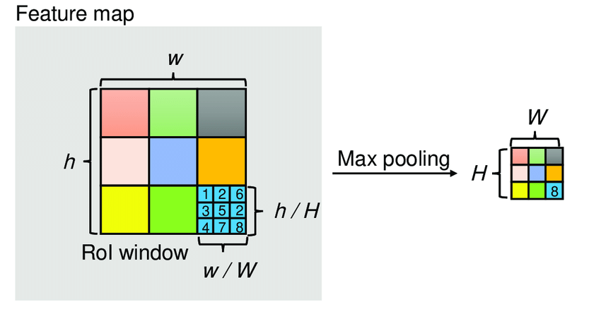
Faster RCNN inherits RoI pooling layer from Fast RCNN to perform such task. The RoI pooling layer uses max pooling to convert feature insides any valid region of interest into a small feature map with a fixed spatial extent of $H \times W$ (eg. $7\times7$), where $H$ and $W$ are layer hyper-parameters that are independent of any particular RoI.
As explained, the feature map was subsampling by $r$ from the original image. It means each coordinate can decreased by $r$ times. The steps are as following.
- RoI pooling is to divide the each coordinate by $r$ and take the integral part: $[\frac{x}{r}]$. After this, the new coordinates reference the feature map, then we could crop feature representation from feature map with the new coordinates.
- For getting a fix-sized output from RoI pooling, cropped part is divided into bins with dimension of $H \times W$. The value of each bin could be taken by either maximum or average.
The RoI max pooling is illustrated in Figure 3.
 Figure 3. RoI Max Pooling Illustration.
class RoIPool(nn.Module):
    """
    RoI Pooling module to get feature extraction for each RoI

    Params:
        pool_height: height of feature extraction of RoI
        pool_width: width of feature extraction of RoI
        spatial_scale: the subsampling scale of feature map compared with original image, which is 1/r
    """
    def __init__(self, pool_height, pool_width, spatial_scale):
        super(RoIPool, self).__init__()
        self.pool_height = pool_height
        self.pool_width = pool_width
        self.spatial_scale = spatial_scale

    def forward(self, features, rois):
        """
        Params:
            features: the feature map with dimension (1, number of channel, height, width)
            rois: the region of interests with dimension (1, number of roi, x_min, y_min, x_max, y_max)
        """
        batch_size, num_channels, fmap_height, fmap_width = features.size()
        num_rois = rois.size()[0]
        outputs = Variable(torch.zeros(num_rois, num_channels, self.pool_height, self.pool_width))

        for roi_idx, roi in enumerate(rois[0,:]):
            roi_start_x_fmap, roi_start_y_fmap, roi_end_x_fmap, roi_end_y_fmap = np.round(roi*self.spatial_scale)
            roi_width_fmap = max(roi_end_x_fmap-roi_start_x_fmap, 1)
            roi_height_fmap = max(roi_end_y_fmap-roi_start_x_fmap,1)

            bin_size_w_fmap = float(roi_width_fmap)/float(self.pool_width)
            bin_size_h_fmap = float(roi_height_fmap)/float(self.pool_height)

            for pool_x_idx in range(self.pool_width):
                bin_x_start = int(np.floor(pool_x_idx*bin_size_w_fmap))
                bin_x_end = int(np.ceil((pool_x_idx+1)*bin_size_w_fmap))

                bin_x_start = min(fmap_width, roi_start_x_fmap+bin_x_start)
                bin_x_end = min(fmap_width, roi_start_x_fmap+bin_x_end)

                for pool_y_idx in range(self.pool_height):
                    bin_y_start = int(np.floor(pool_y_idx*bin_size_h_fmap))
                    bin_y_end = int(np.ceil((pool_y_idx+1)*bin_size_h_fmap))

                    bin_y_start = min(fmap_height, roi_start_y_fmap+bin_y_start)
                    bin_y_end = min(fmap_height, roi_start_y_fmap+bin_y_end)

                    is_empty = (bin_x_end<=bin_x_start) or (bin_y_end<=bin_y_end)
                    if is_empty:
                        outputs[pool_x_idx, pool_y_idx] = 0
                    else:
                        outputs[pool_x_idx, pool_y_idx] = torch.max(features[0,bin_x_start:bin_x_end, bin_y_start:bin_y_end])
        return outputs
Region-based Convolutional Neural Network (RCNN)
RCNN is the final step is the final step in Faster RCNN framework. After getting a feature map from base network, using it to get region proposals with RPN, and standarizing the dimension of feature extraction with RoI pooling, we finally need apply classification on the extracted features. RCNN has two tasks:
- Classify each region proposal into one of the classes (all target classes plus background)
- Finer adjust the bounding box for the region proposals
The original paper takes the max-pooled feature map of each proposal, flatten it and use two fully-connected layer with ReLU activation. Then it uses two differnt fully connected layers for two different tasks aforementioned.
The objective for RCNN is almost the same as RPN. The major difference is that it takes into account the different possible classes.
Training
The original Faster RCNN paper was using multi-step alternating approach to train RPN and RCNN. But after further exploration, nowdays Faster RCNN is trained by end-to-end approach, which leads to better result.
The implementation is straightforward, which wonot be coverd by this article.